Project 1: Nudging algorithm for data assimilation
The goal of this project was to determine efficient algorithms for numerically solving the Navier-Stokes equations. We often see these equations solved analytically with many simplifications yielding an exact solution. We also see the Navier-Stokes equations combined with continuity and energy equations to solve for velocity fields in CFD software. In this project, we use a known velocity field, gathered from Particle Image Velocimetry data to reconstruct the pressure field. This could have useful applications, for example in generating the pressure profile over an airfoil.
The Navier-Stokes equation, in vector form, is:
$$\rho \frac{D\vec v}{Dt} = -\nabla P + \rho \vec g + \mu\nabla^2\vec v$$
Taking the velocity vector to be known, we can then write (in 2D):
$$\frac{\partial P}{\partial x} = f(\vec v), \frac{\partial P}{\partial y} = g(\vec v)$$
This means that \(\frac{\partial P}{\partial x}\), the pressure gradient with respect to \(x\) can be written as a function of the velocity vector \(\vec v\), which is known. The logic follows similarly for \(y\).
We can then solve the pressure gradients numerically, by solving a series of matrix equations. We write the following:
$$\begin{bmatrix} D_{x} \\ D_{y} \\ J\end{bmatrix}
\begin{bmatrix} P_{1} \\ P_{2} \\ \vdots \\ P_{n}\end{bmatrix} =
\begin{bmatrix} f_{1} \\ f_{2} \\ \vdots \\ f_{n} \\ g_{1} \\ g_{2} \\ \vdots \\ g_{n} \\ J_{1} \\ J_{2} \\ \vdots \\ J_{i}\end{bmatrix}$$
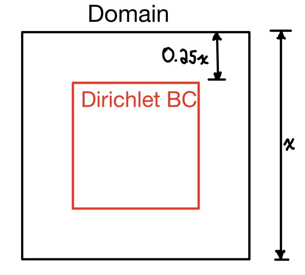
\(D_{x}\) represents the discretized equations representing the pressure gradient with respect to \(x\), while the same logic follows for \(y\). For simplicity, I used the Central Differencing Scheme. The \(P\) vector, \(P = \begin{bmatrix}P_{1} \ P_{2} \ \cdots \ P_{n}\end{bmatrix}^T\) is the pressure field, the solution to the N-S equations that we are seeking. We are trying to solve for \(P\) while minimizing experimental error. The \(J\) matrix represents the known pressure points within the domain. In a practical example, these could be pressure transducers along an airfoil, representing a Dirichlet boundary condition. At least 1 point must be known, otherwise, the matrix will not be full rank, and thus a solution is impossible. \(J\) was the main focus of the project. My role was creating a MATLAB code for solving these equations. I did this by creating a sinusoidal “sample” velocity field to simulate an experiment. I added the generation of Gaussian noise within the velocity field, so we could simulate the effect of experimental error. We found that increasing the number of Dirichlet boundary conditions minimized the error, which makes sense logically. We first tested a square domain, where we found the best position to place the Dirichlet BC’s (pressure transducers) was in the mid-region of the domain, as shown below.
If something about the tendency of the velocity field is known, it is also possible to weight \(D_{x}\), \(D_{y}\), and \(J\) differently to minimize the effect of the Gaussian noise (experimental error). Since the solver used a least squares algorithm (LSQR) in MATLAB for solving the system, weighing portions of the matrix differently represented applying a linear scaling factor to that portion of the matrix. For example, changing the weight of \(D_{x}\) by a factor of \(k\):
$$\begin{bmatrix} kD_{x} \\ D_{y} \\ J\end{bmatrix}
\begin{bmatrix} P_{1} \\ P_{2} \\ \vdots \\ P_{n}\end{bmatrix} =
\begin{bmatrix} kf_{1} \\ kf_{2} \\ \vdots \\ kf_{n} \\ g_{1} \\ g_{2} \\ \vdots \\ g_{n} \\ J_{1} \\ J_{2} \\ \vdots \\ J_{i}\end{bmatrix}$$
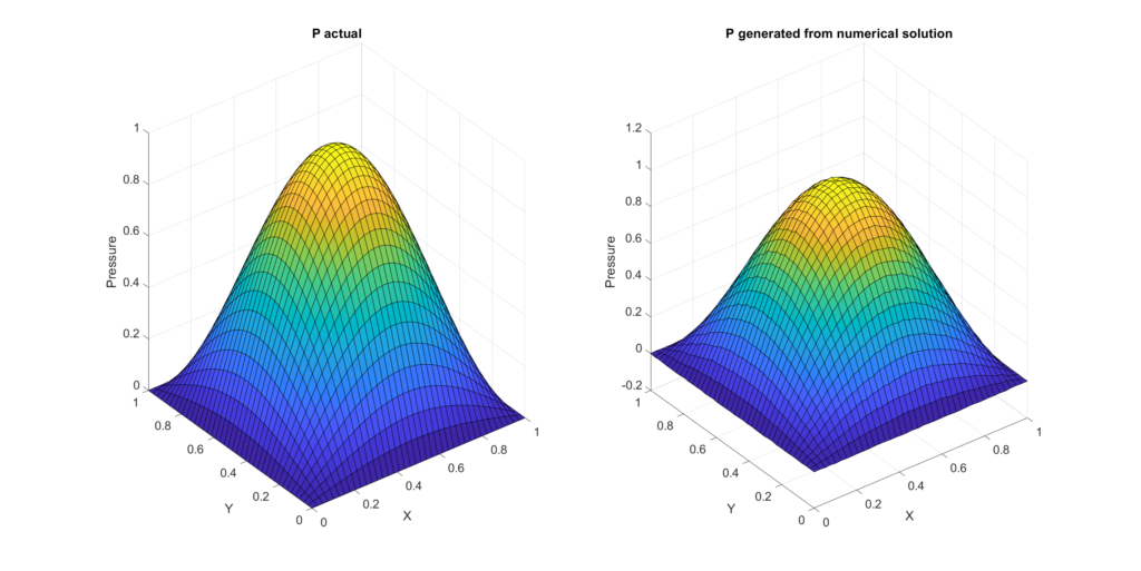
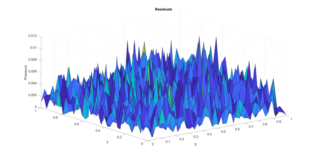
We found that generally, increasing the weight of \(J\) by a factor of 1.2 minimized error, although this was highly dependent on the velocity field. If the velocity field was stronger with respect to either \(x\) or \(y\), the weight of \(D_{x}\) or \(D_{y}\) should be increased to match. For example, if the velocity field was 5x stronger in \(x\), \(D_{x}\) should be weighed 5x greater than \(D_{y}\), assuming that the errors are on the same order of magnitude for both directions. An example solution is shown below. With no Gaussian noise generation, residuals tend to 0 (with some roundoff error).
Project 2: Modelling of Sloshing within a Cone
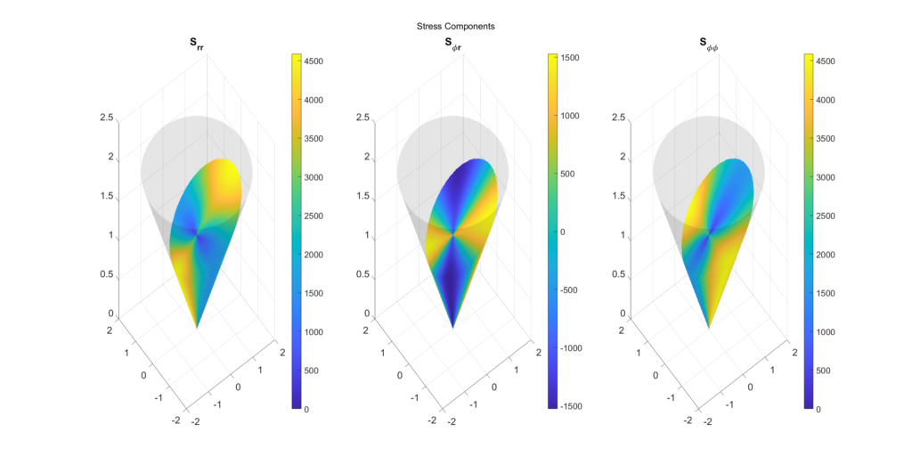
This was a small project where I helped model some of the sloshing dynamics shown here. After conducting a literature review, the fluid motion within the sloshing cone was modelled as a discontinuous function where the water level could be at three different positions, either of the two extremes as well as in the centre. This allowed the stresses within the fluid to be computed by taking the fluid’s motion to be analogous to a wave, where radiation stress is observed due to the excess momentum from a wave. The stresses could be plotted in MATLAB (where \(r\) is the radial direction and \(\phi\) is the tangential direction), shown below, where the stress distribution explains the swirling motions observed on the fluid surface. The stresses are a function of the fluid properties, and wave properties (frequency and amplitude). The stress pattern on the surface is the same for all fluids subjected to a sinusoidal sloshing function.